2. Assignments.

Стр 1 из 22Следующая ⇒

Contents.

1. Introduction. 2

2. Assignments. 6

3. Description of the used methods. 8

4. Progress of work. 11

4. 1. The computer model developed by means subsystem SimEvents. 11

4. 2. Computer model developed by means subsystem StateFlow. 13

5. Results of modeling. 22

5. 1. Results of modeling in subsystem SimEvents. 22

5. 2. Results of modeling in subsystem StateFlow. 22

6. Conclusion. 23

List of references. 24

Attachment №1. 25

Attachment №2. 26

1. Introduction

A mathematical model is a description of a system using mathematical concepts and language. The process of developing a mathematical model is termed mathematical modeling. Mathematical models are used in the natural sciences (such as physics, biology, earth science, meteorology) and engineering disciplines (such as computer science, artificial intelligence), as well as in the social sciences (such as economics, psychology, sociology, political science). Physicists, engineers, statisticians, operations research analysts, and economists use mathematical models most extensively. A model may help to explain a system and to study the effects of different components, and to make predictions about behavior.

Mathematical modeling of queuing consists of modeling the stream of customer entities and modeling the functioning of service channels.

To describe real-world objects functioning under the action of random factors, a class of mathematical models called queuing systems (QS) is often used. The functioning of these objects has the nature of the service of received customer entities or clients.

Queuing system is a mathematical (abstract) object that contains one or more devices D (channels), servicing arrived customer entities E, and storage S, which contains the queue Q of entities waiting for service (Figure 1. 1).

Simulation model of QS is a model that reflects the behavior of the system and changes of its state in time for the given streams of entities arriving on the system inputs. The output parameters are the values that characterize the quality of a system functioning, such as

• utilization coefficients of service channels;

• maximum and average length of the queue in the system;

• time spent by entity in queues and service channels.

To implement discrete-event simulation in Simulink environment is used a SimEvents component. The SimEvents can be used to model and design distributed control systems, hardware configurations, communication networks for the aerospace, automotive, electronics and other applications. You can also simulate event-driven processes, such for example, as a stage of the production process to determine the resource requirements and the estimation of production bottlenecks.

SimEvents and Simulink provide an integrated environment for modeling hybrid dynamic systems containing continuous components and components with discrete events and discrete time.

What does a discrete event simulation mean? In the simulation of discrete events or in event-based modelling the system states are changed due to the occurrence of asynchronous discrete incidents, which called events. In contrast the modelling based solely on differential or difference equations where time is an independent variable is called modelling based on time because the state of the system are time-dependent. Simulink is intended for modeling based on time, while SimEvents was created for discrete event simulation. The choice of the simulation type depends from both exploring phenomenon, and the manner in which it intended to study.

The discrete-event simulation uses the concept of entity. Customer entities can move through the sets of queues (queues), servers (servers) and switchers (switches), controlled by discrete events during the simulation.

Graphical blocks of SimEvents can represent a component that processes customer entities, but entities themselves do not have a graphical representation.

Event – is an instantaneous discrete incident that changes a state variable, an output, and/or the occurrence of other events. Examples of events that can occur during simulation of a SimEvents model are:

· the advancement of an entity from one block to another;

· the completion of service on an entity in a server.

· The SimEvents tools that significantly facilitating the process of simulation of queuing systems in Simulink does not allow to overcome the limits of the algorithms of the separate blocks operation specified by founders. The work with such systems in StateFlow can provide greater flexibility. The StateFlow component is also designed to work with the discrete event systems; however, it allows to model explicitly the blocks and systems states and to define the logical conditions for transitions between the states.

· The StateFlow is a graphical tool for designing the complex control systems, which allows the modeling of behavior of the event driven systems based on Harel statecharts.

· There are two groups of elements at the StateFlow chart – graphic and non-graphic. All the graphic elements are presented on the left panel of the main window – StateFlow Editor. There are " state" (state), " transition" (transition), " default transition" (default transition), " the transition to the last active state" (history junction), " alternative sign" (junction).

· Non-graphic elements of the StateFlow are variables, events and codes. Events, data and codes have no graphic presentation in the StateFlow editor. But you can see them in the StateFlow explorer.

· Events – are the non-graphic objects in the StateFlow which control the chart. The appearance of the event changes the status of the related states and transitions.

Mathematical models can help students understand and explore the meaning of equations or functional relationships. After developing a conceptual model of a physical system it is natural to develop a mathematical model that will allow one to estimate the quantitative behavior of the system.

Quantitative results from mathematical models can easily be compared with observational data to identify a model's strengths and weaknesses.

Mathematical models are an important component of the final " complete model" of a system which is actually a collection of conceptual, physical, mathematical, visualization, and possibly statistical sub-models.

Here we list several examples showing why and when statistical models are useful.

Statistical models or basic statistics can be used:

To characterize numerical data to help one to concisely describe the measurements and to help in the development of conceptual models of a system or process;

To help estimate uncertainties in observational data and uncertainties in calculation based on observational data;

To characterize numerical output from mathematical models to help understand the model behavior and to assess the model's ability to simulate important features of the natural system (model validation). Feeding this information back into the model development process will enhance model performance;

To estimate probabilistic future behavior of a system based on past statistical information, a statistical prediction model.

It is most important to remember that mathematical models are representations or descriptions of reality—by their very nature they depict reality

To extrapolation or interpolation of data based on a linear fit (or some other mathematical fit) are also good examples of statistical prediction models.

To estimate input parameters for more complex mathematical models.

To obtain frequency spectra of observations and model output.

2. Assignments.

Assignments for course work on discipline «Mathematical modeling of objects and control systems»:

The work should be done in two ways:

1) using StateFlow Simulink Matlab subsystem

2) using SimEvents Simulink Matlab subsystem. If necessary, use additional blocks StateFlow and Simulink

Task:

The Poisson stream of details with intensity of 20 details in an hour comes to the factory. With probability 0, 4 detail arrive on the first site, and with probability 0, 6 – on the second site. On the first site of a detail are processed on one of two machines. Holding time has exponential distribution with average value of 48 min. On the second site of a detail process one machine in time which is evenly distributed in the range of 2 ± 1 min. After processing on one of two sites of a detail go to the third site with one machine on which time of processing has exponential distribution with average value of 2 min.

It is necessary to model processing of 1000 details. To define quantity of details which passed through the first site, and the maximum length of turn before the third site.

Our work should be done in two ways:

1) using StateFlow Simulink Matlab subsystem;

2) using SimEvents Simulink Matlab subsystem.

The structure scheme is represented in the Figure 1.

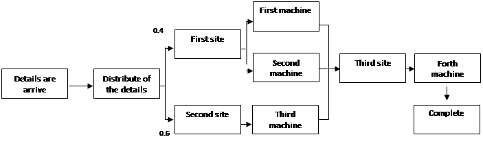
Figure1 Structure scheme of the factory.

The arrows means move of the detail on the shop.

12 3 4 5 6 7 8 9 10 Следующая ⇒