Transition diagram

Аpplication of Markov Chain in business

Markov process fits into many real life scenarios. Any sequence of event that can be approximated by Markov chain assumption, can be predicted using Markov chain algorithm. In the last article, we explained What is a Markov chain and how can we represent it graphically or using Matrices. In this article, we will go a step further and leverage this technique to draw useful business inferences.

“Krazy Bank”, deals with both asset and liability products in retail bank industry. A big portfolio of the bank is based on loans. These loans make the majority of the total revenue earned by the bank. Hence, it is very essential for the bank to find the proportion of loans which have a high propensity to be paid in full and those which will finally become Bad loans. “Krazy Bank” has hired you as a consultant to come up with these scoping numbers.

All the loans, which have been issued by “Krazy Bank” can be classified into four categories:

1. Good Loans: These are the loans which are in progress but are given to low risk customers. We expect most of these loans will be paid up in full with time.

2. Risky loans: These are also the loans which are in progress but are given to medium or high risk customers. We expect a good number of these customers will default.

3. Bad loans: The customer to whom these loans were given have already defaulted.

4. Paid up loans: These loans have already been paid in full hort Note on Absorbing nodes

Absorbing nodes in a Markov chain are the possible end states. All nodes in Markov chain have an array of transitional probability to all other nodes and themselves. But, absorbing nodes have no transitional probability to any other node. Hence, if any individual lands up to this state, he will stick to this node for ever. Let’s take a simple example. We are making a Markov chain for a bill which is being passed in parliament house. It has a sequence of steps to follow, but the end states are always either it becomes a law or it is scrapped. These two are said to be absorbing nodes. For the loans example, bad loans and paid up loans are end states and hence absorbing nodes.

Transition diagram

You have done a thorough research on past trends of loan cycle and based on past trends here is the Markov chain you observed (for a period of 1 year):

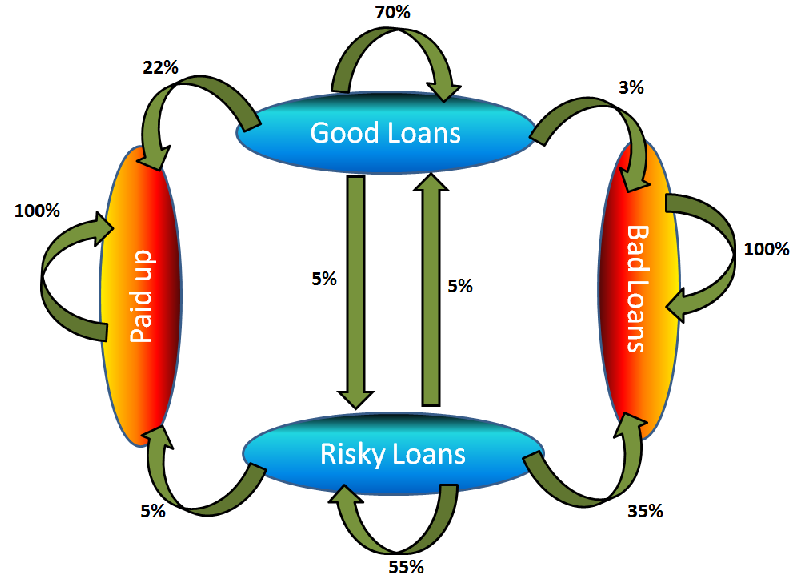
Explaining absorbing nodes becomes simple from this diagram. As you can see, Paid up and bad loans transition only to themselves. Hence, whatever path a process takes, if it lands up to one of these two states, it will stay there for ever. In other words, a bad loan cannot become paid up, risky or good loan ever after. Same is true with paid up loans.

Tra Once, we have 1 year transition probability, we can convert prediction algorithm to simple matrix multiplication. Currently the portfolio has 60% Good and 40% Risky loans. We look forward to calculate, how many of these loans will be finally paid up in full? Using 1 year transition probability, we can estimate the number of loans falling into each of the four bucket 1 year down the line.

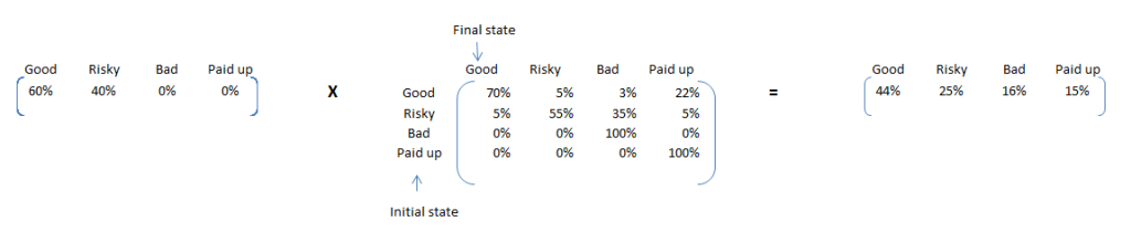
Here are some interesting insights from this calculation. We can expect 15% of the loans to be paid up in this year and 16% being ending up as bad loans. As the % of bad loans seem to be on a higher side, it will be beneficial to identify these loans and make adequate interventions. Pin pointing to these 15% is not possible using simple Markov chain, but same is possible using a Latent Markov model.

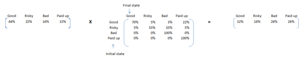
Now, to make a prediction for 2 years, we can use the same transition matrix. This time the initial proportions will the final proportions of last calculation. Transition probability generally do not change much. This is because, it is based on several time points in past.

If we keep on repeating this exercise, we see the proportion matrix converges. Following is the converged matrix. Note that, multiplying it with transition matrix makes no change to proportions.

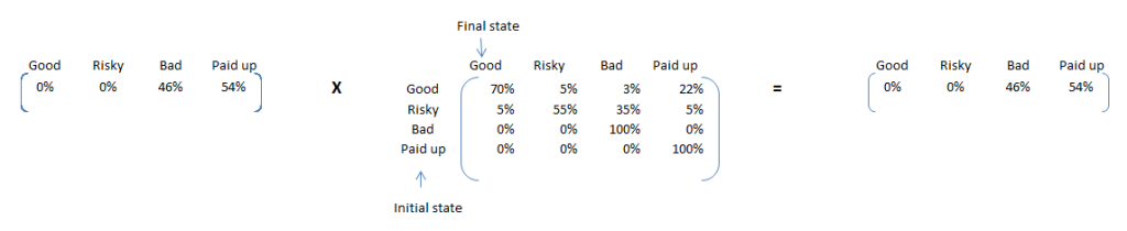
These are the proportion numbers we were looking for. 54% of the current loans will be paid up in full but 46% will default. Hence doing this simple exercise lead us to such an important conclusion that the current portfolio exposes bank to a very high risk.

Lo We have already seen the stationary point proportions for the portfolio. Something which will be of interest to us next is that what proportion of Good loans land up being paid up in full. For this we can start with an initial proportion split of Good – 100% and rest – 0%. Thefinalconvergedmatrixisasfollows:

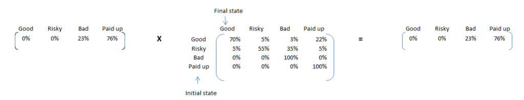
Here are some interesting insights. If the entire portfolio was built of good loans, only 23% of loans would have defaulted against 46% for current portfolio. Hence, we will expect a very high proportion of risky loans will show default. We can find this using a simple transition calculation using Risky – 100% and rest – 0%. Following is the final converged matrix:

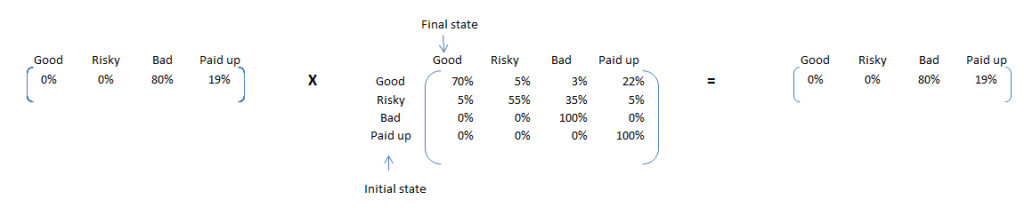80% of such loans will default. Hence, our classification of Risky and Good separates out propensity to default pretty nicely.

⇐ Предыдущая 123 4 5 6 Следующая ⇒